Chapter Five: Digital Audio

5. Sampling Rates | Page 2
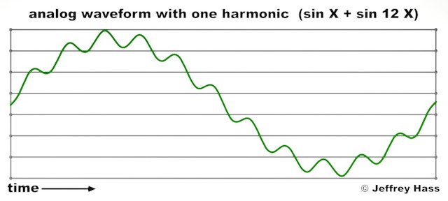
The diagrams below illustrates the effect of two different sampling rates on a single complex periodic waveform which contains both a fundamental frequency and the 12th partial above it (three 8ves and a 5th above the fundamental), resulting in the small nooks and crannies around a sine wave. If the fundamental were A 880 Hz, then the 12th partial would be E 10,560 Hz. According to the Nyquist Theorem, the sampling rate would need to be above the 21,120 samples per second if one wished to represent the upper partial without aliasing. This might be close to the common 22,050 sampling rate of olden days. The examples below are a graphic illustration of how the sampling rate determines the frequency response of a system.
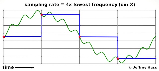
Pictured below, at a sampling rate of four times the fundamental frequency (3,520 samples per second if the fundamental were A880), represented by the red spheres, one is able to digitally represent the fundamental frequency (indicated by the heavier blue lines) but not the higher partial, which would alias if not filtered out prior to entering the system. This demonstrates a very limited frequency response at a low sample rate.
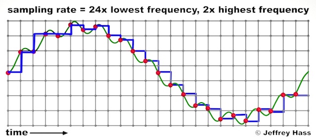
Pictured below is the same waveform (A880+E10,560) sampled at just 2x the highest frequency, which is 21,120 samples per second. Notice ('cause we got lucky), it just barely represents both the fundamental AND the upper partial, represented by the digitized blue line.
In a real-world analog-to-digital conversion, as pitches get higher, more and more of their upper partials both leave the audio range, and exceed the Nyquist frequency. These would be filtered out, even if they could be reproduced. Just one octave higher for our example, and the 12th partial of A1,760, which would be E21,120 would be out audio range, though at a 44.1K sampling rate, would still not alias.
