Chapter Four: Synthesis

Bessel Functions and Sideband Strength

As I increases, each sideband pair follows its own path of increasing and decreasing strength called a Bessel function. The Bessel function curves followed are different for each of the n^th-order sidebands—one of the things that makes frequency modulation so interesting. To trig students, these are called Bessel functions of the first kind of order n; to non-trig students, it's more like Close Encounters of the Third Kind. Below is a graph of the first seven orders (beginning with n=0) of sideband pairs, showing their relative strength on the vertical axis as I increases on the horizontal axis.

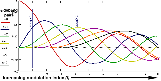
Note that at I = 0 (i.e. no modulation), the carrier (red, n=0) is at full strength. As I increases, several things happen. Firstly, the carrier loses strength, and secondly, each additional order of sideband pairs begins to be heard one by one. A good rule of thumb for predicting how many sideband pairs (n) will be audible for a given value of I is: n = I + 1 with I being rounded off to the nearest integer. Each pair, after its initial peak, will decrease in strength and, for a given value of I, be inaudible as it crosses zero. On the negative side of zero, it will be in reverse phase to any similar frequency on the positive side of zero. To make matters slightly more complicated, each odd-numbered lower sideband (n=1,3,5,...) follows the inverse of the Bessel function associated with it's pair (equivalent to multiplying its strength by -1). As well, each reflected sideband follows the inverse of its Bessel function. And finally, each odd-numbered lower sideband that is reflected follows the given phase of the Bessel function as charted above.

The video below visually and audibly demonstrates the first 6 orders (0-5) of sidebands as I increases from 0 (i.e. no modulation) to 5. The carrier frequency is 700 Hz and the modulating frequency is 85 Hz. See if you can aurally track individual frequencies, such as the carrier (red) as they increase, decrease or disappear as I increases. As sidebands enter the negative domain, indicating their phase has shifted 180 degrees, they appear below the center horizontal frequency line. For the odd-numbers lower sidebands, they track the reverse phase of their positive counterpart, and so as their order of Bessel function dips into negative strength, they appear as the mirrored positive counterpart. You can stop and scrub through the video to get a better look at the timbral dynamic. BTW, moderate your volume level before playing.

Two Examples

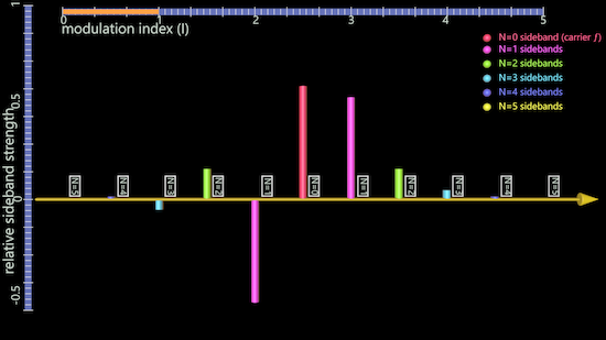
Here are two examples of the spectra produced for fixed values of I, computed by simply looking at the vertical example lines above. The first value of I is relatively low (at a mod index of 1), so only a few sidebands are audible.

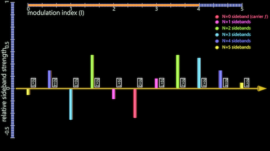
The second example shows a higher value of I at a mod index of 4, which also includes some negative strengths where the Bessel function has dipped below 0. Note, for example, that the n=0 carrier frequency is now in inverted phase.

In general, as I increases, we can infer that more and more frequencies become audible. This can be a problem for digital synthesis, where the upper sidebands may reach the Nyquist frequency (see the digital audio chapter) and alias. FM is not band-limited. For this reason, most digital synthesis will have a limit on the maximum value of I.

Here are two audio examples. The first has a C:M ratio of 1:2 creating a harmonic spectrum, the second a C:M ratio of 1:1.31 creating an inharmonic spectrum. In both examples, the modulation index is increased slowly over 10 seconds from 0 (no modulation) to 15. Play these several times and focus on different frequencies as they move through their Bessel functions. Start with the carrier frequency (the first frequency you will hear). Listen as it immediately begins to lose strength, completely disappears and then reappears. Listen to the effects of phase cancellation in the first harmonic example, which will have far fewer discreet frequencies than the inharmonic one.